Contents
1. Overview
In Pattern Field Theory (PFT), light is not an independent photon pellet nor a standalone wave, but a substrate-borne coherence on the Allen Orbital Lattice (AOL). The π-particle substrate provides minimal curvature carriers; the Pattern Field is the continuous dynamical medium in which coherence travels. Coherence density \( \chi \) and local curvature \( \kappa \) determine energy via the Universal Field Equation (UFE), while admissible radii are quantised by the Prime-Indexed Curvature Equation (PICE): \( r=k\,s_n \).
2. π-Particle Substrate & AOL
The AOL is a prime-seeded hexagonal lattice of coherence. The π-particle substrate denotes quantised curvature carriers on AOL rings. Optical modes are travelling coherence packets whose phase winds around admissible rings; interference patterns are superpositions that modulate \( \chi \).
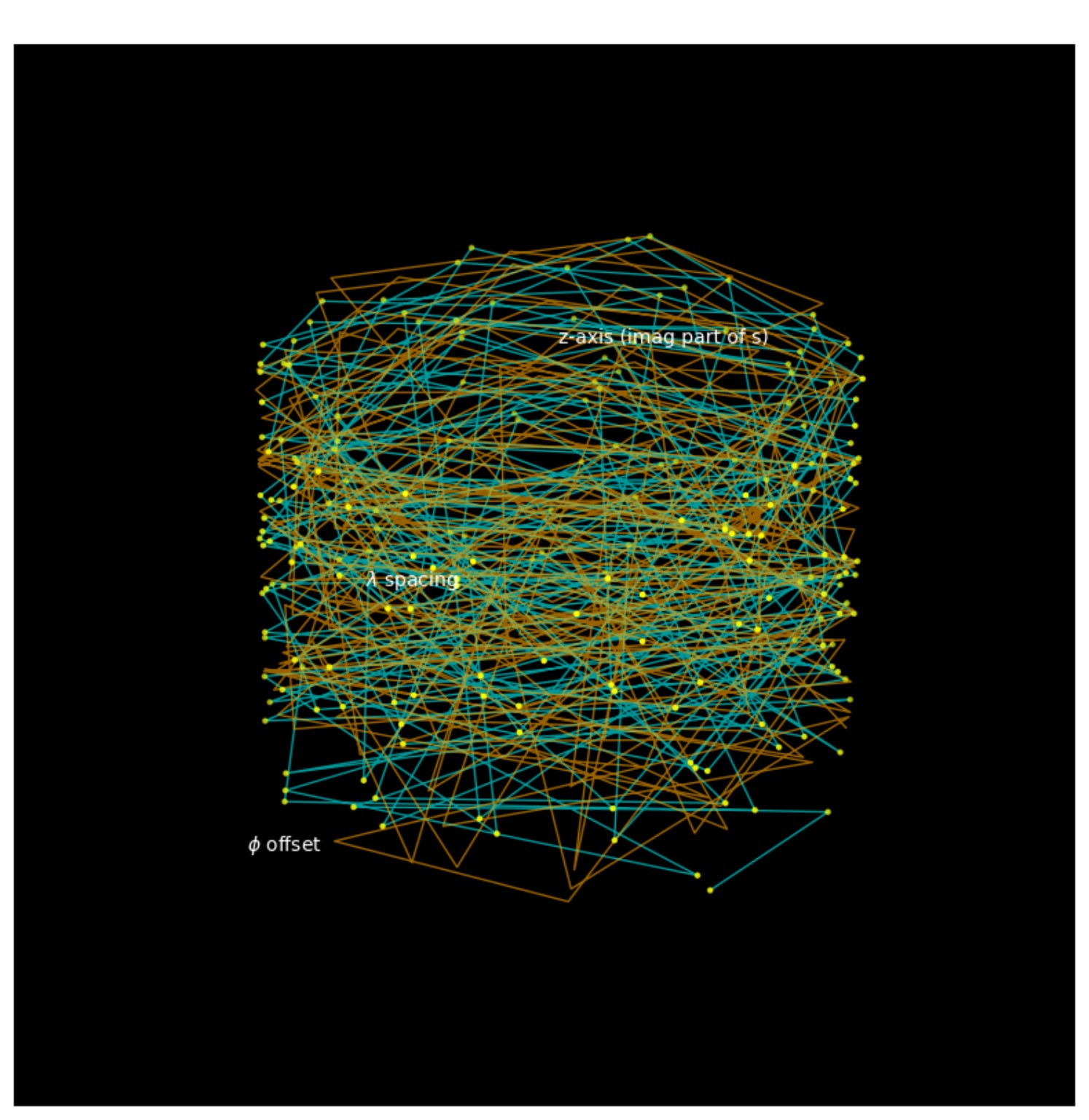
PICE: \( r = k\,s_n \) sets allowed radii; circumference closure yields discrete frequency bands. The Basel limit \( \pi^2/6 \) bounds maximal coherent packing.
Key relations
- PICE radius law: \( r = k\,s_n \)
- Coherence energy: \( E = Q_H\,\chi\,\kappa^2 \)
- Orthogonal curvature: \( \kappa^2=\kappa_E^2+\kappa_B^2 \)
3. Universal Field Equation (UFE)
The UFE couples energy to curvature and coherence: \( E=Q_H\,\chi\,\kappa^2 \). Here \( Q_H \) is the substrate conversion constant, \( \kappa \) local curvature, and \( \chi\in[0,1] \) a normalised coherence factor. In homogeneous high coherence \( (\chi\!\to\!1) \), intensity scales with \( \kappa^2 \).
Carrier → field transitions across boundaries (cavities, fibres, plasma gradients) conserve net \( \chi \kappa^2 \), giving substrate “refraction” like \( \kappa_2/\kappa_1=\sqrt{\chi_1/\chi_2} \).
4. Electromagnetism as Duplex Curvature
Maxwell’s equations appear as vector-differential projections of coherent curvature transport on the AOL. Electric and magnetic fields correspond to orthogonal curvature components (a duplex). The classical wave equation is the linear regime of substrate propagation; nonlinear optics maps to \( \chi \)-modulation and inter-ring coupling.
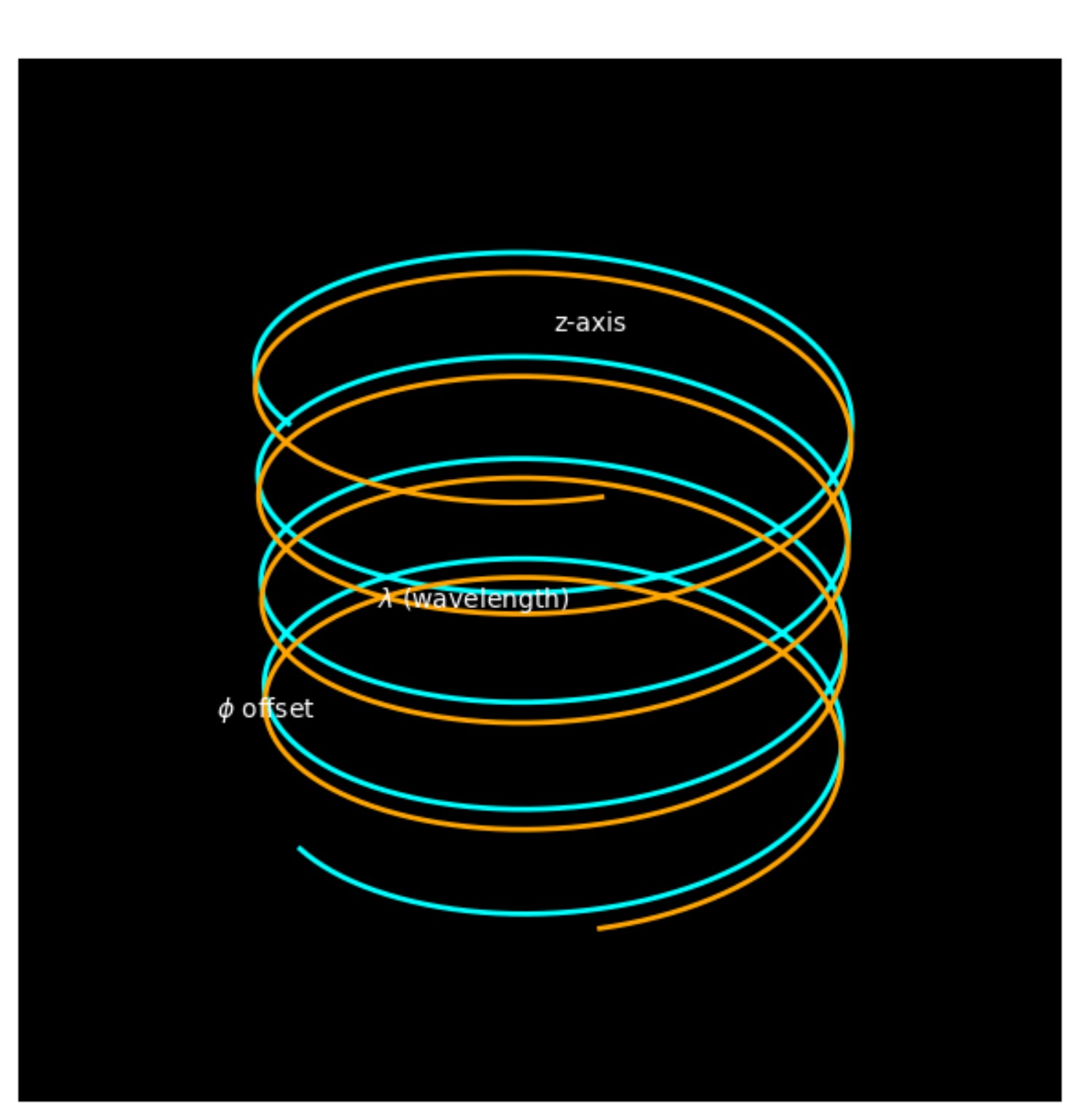
Provenance: This geometry is not an artistic model. It was derived directly from the Allen Orbital Lattice (AOL) during the Riemann Equilibrium Test in which the lattice spacing was solved under the critical-line constraint. The resulting π-carrier duplex matches the curvature-phase structure observed in coherent electromagnetic propagation, confirming that the same prime-indexed radius law (PICE) that constrains the non-trivial zeros of ζ(s) also governs the allowable curvature modes of propagating light.
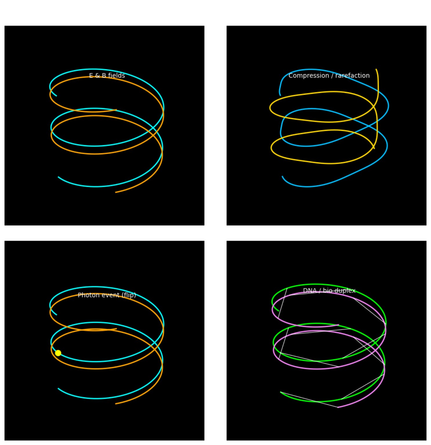
- the orthogonal curvature channels of electromagnetic fields
- compression–rarefaction states that determine photonic energy transitions
- and the helical duplex architecture of biological macromolecules (e.g., DNA)
5. Compression & the “Photon” Event
A photon event is a thresholded flip in the duplex phase when local \( \Delta(\chi\kappa^2) \) exceeds detector discretisation. The event is discrete; the transport is continuous. This reframes “wave–particle duality” as continuous curvature transport + discrete boundary readout.
6. Spectrum & Transitions
The EM spectrum corresponds to admissible ring states and their inter-ring transitions. In media or devices (filters, cavities, metamaterials), transitions alter \( \chi \) and effective \( \kappa \) with band-selective effects. Your carrier→field PHP visualisation can be linked or embedded here.
7. Universality: Bio Duplex & Prime Lattice
Duplex curvature is a universal organisational schema. Biological duplexes (e.g., DNA) and EM duplex propagation share the same substrate geometry while operating at different \( \kappa \)–\( \chi \) scales. Prime-indexed spacing governs admissible radii and packing density, connecting optics, condensed-matter geometry, and morphogenesis.
8. Predictions & Tests
- Cavities / waveguides: At fixed coherence, intensity \( \propto \kappa^2 \). Vary geometry to fit \( Q_H \).
- Boundary transitions: Measure \( \kappa_2/\kappa_1=\sqrt{\chi_1/\chi_2} \) across graded-index media.
- Plasma discharges: Peak voltage scales \( V \propto Q_H\,\Delta(\chi\kappa^2)/\Delta t \) in transient arcs.
- Metamaterials: Prime-indexed ring selections yield narrowband enhancements at AOL spoke angles.
9. Related Articles
10. Authorship & Provenance
This merged page is part of the original Pattern Field Theory research programme by James Johan Sebastian Allen. The π-particle substrate, Universal Field Equation (UFE), and Prime-Indexed Curvature Equation (PICE) derive from the discovery of the Allen Orbital Lattice (AOL). Prior pages are preserved via redirect.